
 Krzysztof Burejza
Problem
The symptom is always similar. A job that usually takes minutes hangs on 199 of 200 tasks: one task has run for a quarter of an hour, the others finished in seconds. Or the job fails with OOM on one executor while the rest of the cluster has free memory.
A typical skew demo gives 90% of the fact rows one customer key on purpose. That shows the mechanism, but in practice someone hears "skew", pastes salting from the internet, and the cause was a join explosion or thousands of empty keys that only needed filtering out.
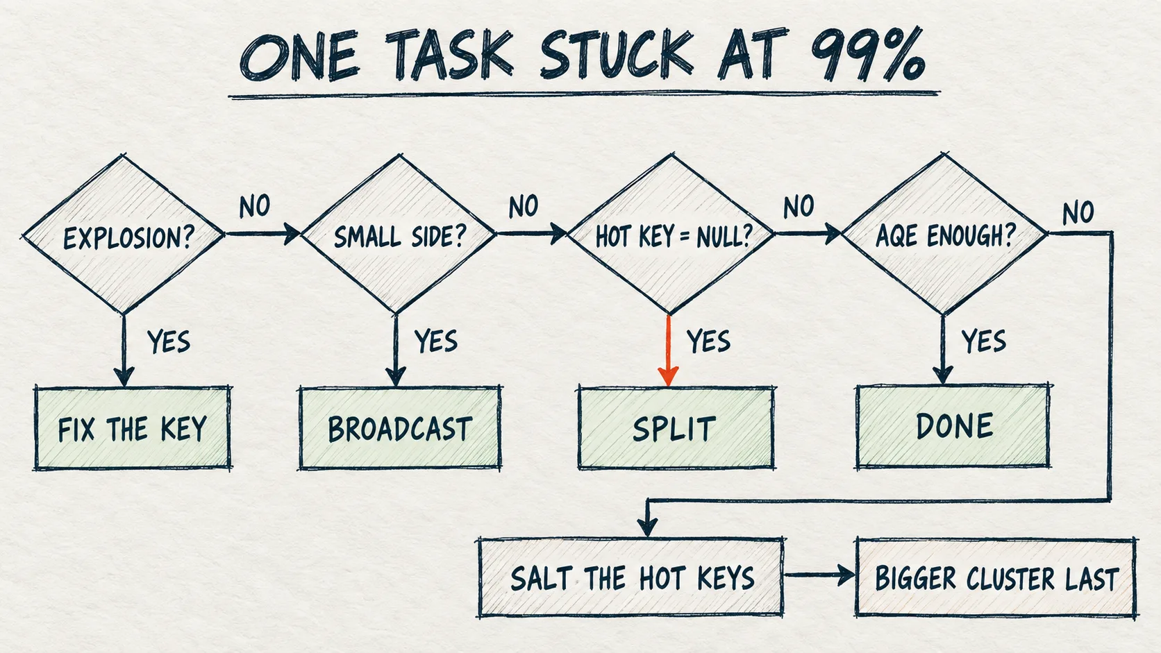
In one project the most skewed key was client_id: one client had 800k orders, the others around 20k each. The fix went in two steps, as in the tree below: first AQE, which splits a skewed join partition on its own, and only when that wasn't enough, salting just the hot key.
How it works
A shuffle spreads rows across partitions by key hash. All rows with one key land in one partition, processed by one task. If CUST000001 holds 90% of the rows, one task gets 90% of the work, however many cores we have.
Spark has three built-in mechanisms for this, each with limits:
| Mechanism | What it does | What it does not do |
|---|---|---|
| AQE skew join | Splits an oversized join partition into several tasks and duplicates the matching partition of the other side for them | Works only for joins with a shuffle. The partition must be both 5× larger than the median and larger than 256 MB (default thresholds per the docs; not readable on serverless). Does not apply to FULL OUTER JOIN, and in a LEFT OUTER join it splits only the left side (in RIGHT OUTER only the right) |
| Partial aggregation | A groupBy with sum, count, max computes a partial result in each task before the shuffle, so the hot key sends one row per task |
Does not reduce the data when the partial result has to keep every element (collect_list, exact percentiles). Window functions are a separate case (step 6) |
| Broadcast join | The small side goes whole to every executor, the large side is not shuffled | Needs a small side. Spark's static threshold (spark.sql.autoBroadcastJoinThreshold) defaults to 10 MB; the runtime threshold at which AQE on Databricks switches to broadcast (spark.databricks.adaptive.autoBroadcastJoinThreshold) is 30 MB |
So on small data AQE won't treat a partition as skewed even with 90% of the rows, as it usually stays under 256 MB after the shuffle. On large data AQE has often solved it, so the problem lives in the middle: a few GB on the hot key, an aggregation whose partial result does not shrink, or a join AQE does not handle.
Classic cluster or serverless: what changes for skew
| Classic cluster (per the docs) | Serverless | |
|---|---|---|
| How work is spread across tasks | Spark UI → Stages → "Summary metrics for tasks", compare the maximum with the 75th percentile | No Spark UI. The query profile can raise a DATA_SKEW insight, and we check the key distribution with a GROUP BY ... ORDER BY cnt DESC query |
AQE thresholds (skewedPartitionFactor, skewedPartitionThresholdInBytes) |
we can read and change them with spark.conf.set |
we can't change them. In the lab spark.conf.get raised AnalysisException for every AQE key we checked |
Broadcast threshold (autoBroadcastJoinThreshold) |
we set it ourselves | not a supported config, so only broadcast hints remain |
spark.sql.shuffle.partitions |
200 by default | auto by default (per spark.conf.get in the lab); our sort-merge join used 21 shuffle partitions (16 on Free Edition) |
| Machine size and type | we choose, including bigger workers | we don't choose, serverless scales on its own |
So on a classic cluster we can tune AQE first; on serverless we go straight to the code: a broadcast hint, splitting out the NULLs, and salting. All results here are from serverless; what I write about classic clusters (Spark UI, AQE thresholds) comes from the docs, not my own test.
When migrating to serverless, remove reads of unsupported settings, because the notebook stops at the first one: [CONFIG_NOT_AVAILABLE.WITHOUT_SUGGESTION] Configuration spark.sql.adaptive.enabled is not available. Also, according to the docs, queries in a serverless job have no default timeout (the 2.5 h default is for notebooks only), so protect a job that can hang with spark.databricks.execution.timeout (in seconds).
The decision tree
0. Is it really skew?
Three problems look alike in the logs but need different fixes:
- Join explosion: the output has many times more rows than the input. It can hit a single key, since 10k occurrences on each side means 100M matches and one very slow task, so we check the key's cardinality on both sides and the output row count. Explosion and skew can happen together, and an explosion is fixed by the join key, not compute.
- Spill in all tasks: partitions are too big for memory, but even. More partitions or earlier filtering helps.
- Skew: one task (or a few) takes clearly longer than the rest.
In the Spark UI the Databricks guide treats a stage as suspicious when the max is 50% or more above the 75th percentile. On serverless the query profile (the See performance link under the cell) can, per the docs, report EXPLODING_JOIN, a join that produces far more rows than it reads, besides DATA_SKEW. The insights don't name the key, so we check the distribution with a query. In the code FACTS and DIM are the tables <catalog>.<schema>.skew_facts and skew_dim (by default workspace.dataistheway), and facts and dim are their DataFrames.
✓ Tested on Free Edition (2026-10-19)
display(spark.sql(f"""
SELECT customer_id,
       count(*)                                         AS cnt,
       round(100 * count(*) / sum(count(*)) OVER (), 2) AS pct
FROM {FACTS}
GROUP BY customer_id
ORDER BY cnt DESC
LIMIT 20
"""))
If the first row holds a large share and the second a fraction of a percent, we have a hot key; if the first row is NULL, go to step 3.
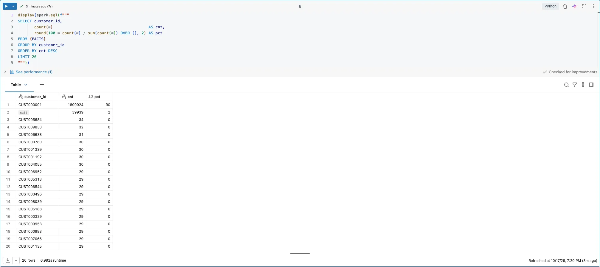
Lab result: the top rows of the key distribution query.
1. Where does the hot key live?
Each operation has a different remedy:
- join → steps 2–5,
groupBy→ step 6,- a window function with
PARTITION BYon the hot key → step 6, - reading files, e.g. one large file in a format that cannot be split, next to many small ones → step 7.
2. Is one side of the join small?
If so, a broadcast fixes it at the root: the large side is not shuffled, so there is no hot partition. AQE picks a broadcast itself when a side turns out small after filters, and on serverless we can force it only with a hint.
✓ Tested on Free Edition (2026-10-19)
bc = spark.sql(f"""
SELECT /*+ BROADCAST(d) */ f.*, d.segment
FROM {FACTS} f
JOIN {DIM} d ON f.customer_id = d.customer_id
""")
print("rows:", bc.count())
bc.explain()
In the lab the plan showed a PhotonBroadcastHashJoin with no fact-side shuffle, and the join returned 1,960,061 rows, i.e. 2M minus the NULLs. The broadcast side must fit in every executor's memory, though, so a large, wide dimension is an OOM risk on the driver and executors.
3. Is the hot key NULL?
The most common "skew", and it needs no salting. It depends on the join type:
- In an inner join the optimiser adds an
isnotnull(key)filter on both sides, since NULL never satisfies equality, so NULL rows never reach the shuffle. Check it in the plan rather than adding the filter blindly. - In left, right and full outer joins NULL rows must stay in the result, so they all land in one partition. The popular line that "NULLs never match in inner/left join anyway" is wrong here: in a left join NULLs do not match, but they do not disappear.
✓ Tested on Free Edition (2026-10-19)
facts.join(dim.hint("merge"), "customer_id", "inner").explain()
The inner join plan had the isnotnull(customer_id) filter on both sides, so 39,939 NULLs were dropped before the shuffle.
For an outer join, cut the NULLs off before the join and append them back with empty dimension columns.
✓ Tested on Free Edition (2026-10-19)
nulls    = facts.filter(F.col("customer_id").isNull())
nonnulls = facts.filter(F.col("customer_id").isNotNull())

dim_cols = [c for c in dim.columns if c != "customer_id"]
left_joined = (
    nonnulls.join(dim, "customer_id", "left")
    .unionByName(nulls.select("*", *[F.lit(None).cast(dim.schema[c].dataType).alias(c)
                                     for c in dim_cols]))
)

plain_left = facts.join(dim, "customer_id", "left")
print("facts:", facts.count(), "| left_joined:", left_joined.count(), "| plain left join:", plain_left.count())
assert left_joined.count() == facts.count() == plain_left.count()
With a unique key in the dimension the row count must match facts.count(); in the lab both versions returned 2,000,000 rows. The same applies to a groupBy on a column with many NULLs: the NULL group is one group and one task.
4. Is AQE already coping?
AQE is on by default on Databricks and splits a hot partition above the table's thresholds by itself. On a classic cluster the Spark UI (SQL/DataFrame tab) shows isSkew=true on the SortMergeJoin node, and you can lower the thresholds. On serverless we can neither change nor read them, and I did not see the split in the lab either, because explain() over Spark Connect shows a plan analysed from scratch (always AdaptiveSparkPlan with isFinalPlan=false).
✓ Tested on Free Edition (2026-10-19)
# AQE settings (usually not readable on serverless)
for k in ["spark.databricks.optimizer.adaptive.enabled",
          "spark.sql.adaptive.enabled",
          "spark.sql.adaptive.skewJoin.enabled",
          "spark.sql.adaptive.skewJoin.skewedPartitionFactor",
          "spark.sql.adaptive.skewJoin.skewedPartitionThresholdInBytes",
          "spark.sql.shuffle.partitions"]:
    try:
        print(f"{k:62s} = {spark.conf.get(k)}")
    except Exception as e:
        print(f"{k:62s} = not available ({type(e).__name__})")
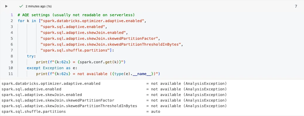
Lab result: reading the AQE settings with spark.conf.get on serverless.
The second condition is the join type. AQE splits a skewed partition on both sides of an inner or cross join, only on the left side of a left outer, left semi or left anti join, only on the right side of a right outer join, and does not optimise a full outer join at all. If the hot key sits on an unsupported side, swapping sides does not help, because the preserved side stays the same; what remains is changing the join type, broadcast or salting.
If a job hangs on one task with AQE on, the operation is not a join, the join is not supported, the partition is under the threshold, or the hot key is too big even after the split, and we move on to salting. Instead of the older SKEW hint, the docs now recommend AQE skew handling, which is usually faster.
5. Salting: hot keys only
Salting splits a hot key into N sub-keys. Each hot-key fact row gets a random salt from 0 to N−1, that key's dimension row is duplicated N times, once per salt, and the join runs on (key, salt). A common rule of thumb: salting makes sense when AQE is not enough and the key imbalance exceeds 100:1.
✓ Tested on Free Edition (2026-10-19)
import time

t0 = time.time()
plain_cnt = facts.join(dim.hint("merge"), "customer_id").count()
t_plain = time.time() - t0

N = 16
hot_keys = [r["customer_id"] for r in
            facts.groupBy("customer_id").count()
                 .filter("count > 100000").select("customer_id").collect()]
print("hot keys:", hot_keys)

facts_s = facts.withColumn(
    "salt",
    F.when(F.col("customer_id").isin(hot_keys), (F.rand() * N).cast("int"))
     .otherwise(F.lit(0)))

dim_s = (dim.withColumn(
            "salts",
            F.when(F.col("customer_id").isin(hot_keys), F.sequence(F.lit(0), F.lit(N - 1)))
             .otherwise(F.array(F.lit(0))))
            .withColumn("salt", F.explode("salts"))
            .drop("salts"))

t0 = time.time()
salted = facts_s.join(dim_s.hint("merge"), ["customer_id", "salt"]).drop("salt")
salted_cnt = salted.count()
t_salted = time.time() - t0

print(f"plain join  : {plain_cnt} rows, {t_plain:.1f}s")
print(f"salting     : {salted_cnt} rows, {t_salted:.1f}s")
assert plain_cnt == salted_cnt, "salted join changed the row count"
The merge hint forces a sort-merge join so the small demo dimension is not broadcast (real salting does not need it), but Photon reported the SortMergeJoin node as unsupported, so such a join runs outside Photon. The hot key threshold (count > 100000) is better relative, e.g. the share from step 0. We do not salt NULLs, since isin() will not match them; step 3 handles them.
In the lab the only hot key was CUST000001, and 1.6 s versus 1.5 s is noise (in other runs either one won), since at 2M rows skew does not hurt yet.
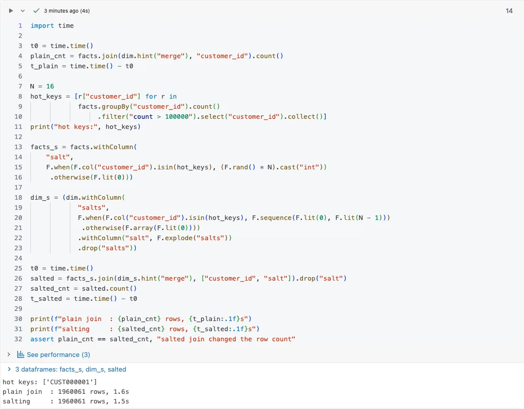
Lab result: the plain join and the salted join, both with the merge hint.
Salting shows in the row distribution:
✓ Tested on Free Edition (2026-10-19)
# Row distribution after salting (an approximation of what each task gets)
display(facts_s.groupBy("customer_id", "salt").count().orderBy(F.desc("count")).limit(20))
Each (key, salt) pair is roughly one join task's work, so instead of 1,800,024 rows under one key we get 16 pairs of about 112k rows.
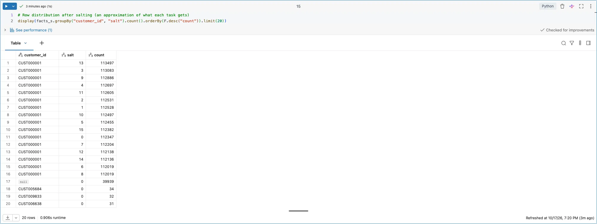
Lab result: rows per (key, salt) pair after salting.
Since Photon does not support SortMergeJoin, shuffle_hash is the better hint there: it also forces a shuffle, but the join stays in Photon, and AQE handles skew in a shuffle hash join too. For timing, a few writes to the noop sink beat count(), which lets Spark skip columns it does not need to count rows.
✓ Tested on Free Edition (2026-10-19)
# The same two joins with shuffle_hash instead of merge, timed with the noop sink (3 runs each)
for name, df in [("plain join", facts.join(dim.hint("shuffle_hash"), "customer_id")),
                 ("salting", facts_s.join(dim_s.hint("shuffle_hash"), ["customer_id", "salt"]))]:
    times = []
    for _ in range(3):
        t0 = time.time()
        df.write.format("noop").mode("overwrite").save()
        times.append(round(time.time() - t0, 1))
    print(f"{name:12s}: {times} s")
df.explain()
In the lab the plan had a PhotonShuffledHashJoin node ("The query is fully supported by Photon"), and the two variants differed by tenths of a second that changed between runs.
Salting costs code to maintain, a hot key list that changes, and duplicated dimension rows, so it sits late in the tree.
6. Skewed groupBy and window functions
The popular "repartition() + salting" advice for a skewed groupBy mixes up two things. A repartition() on the same key hurts, because there is no partial aggregation before that shuffle, as the plan shows:
✓ Tested on Free Edition (2026-10-19)
# repartition() by the key before groupBy: where does the partial aggregation go?
facts.repartition("customer_id").groupBy("customer_id").agg(F.sum("amount")).explain()
facts.groupBy("customer_id").agg(F.sum("amount")).explain()
In the lab the first plan had no aggregation before the REPARTITION_BY_COL shuffle, so all 1,800,024 hot-key rows went to one partition; in the second partial_sum(amount) runs in every task before the shuffle.
Salting an aggregation works differently: aggregate by (key, salt), then merge by the key alone. So the question is whether partial aggregation shrinks the hot key's data:
- With
sum,count,min,maxandavgit already does, so a second salted stage is usually wasted work. - Spark plans
count(DISTINCT x)in several steps on its own (first removing duplicate (key, x) pairs in each task), so splitting it by hand intodistinct()andcountis not an optimisation. - Two-stage salting helps when there is no partial aggregation before the hot partition, e.g. right after a join on the same key or with
applyInPandas. Withcollect_listthe second stage still gathers everything into one task. - A window function
row_number() OVER (PARTITION BY customer_id ORDER BY ts)sorts all rows of the key in one task.max_bygives the latest row per key with partial aggregation, and since it picks any row on anorder_tstie, a pipeline adds a tie-breaker, e.g.F.struct("order_ts", "order_id")as the second argument.
✓ Tested on Free Edition (2026-10-19)
# count(DISTINCT product_id) per customer: what Spark plans on its own
direct = facts.groupBy("customer_id").agg(F.countDistinct("product_id").alias("count"))

# the same written by hand in two steps; count("product_id") skips NULL like count(DISTINCT) does
two_step = (facts.select("customer_id", "product_id").distinct()
                 .groupBy("customer_id").agg(F.count("product_id").alias("count")))

print("rows that differ:", two_step.exceptAll(direct).count() + direct.exceptAll(two_step).count())

# compare the physical plans: look for an aggregate keyed by (customer_id, product_id) in both
direct.explain()
two_step.explain()
In the lab both versions gave the same plan (a PhotonGroupingAgg on (customer_id, product_id) before the shuffle) and result. Spark without Photon may shuffle by the pair first, which does not change the conclusion. The manual version makes a NULL mistake easy, though:
✓ Tested on Free Edition (2026-10-19)
# NULL check: products [7, 7, NULL] -> count(DISTINCT) = 1; .count() after distinct() would give 2
t = spark.createDataFrame([("C1", 7), ("C1", 7), ("C1", None), ("C2", None)], "customer_id string, product_id int")
display(t.groupBy("customer_id").agg(F.countDistinct("product_id").alias("count_distinct"))
         .join(t.distinct().groupBy("customer_id").agg(F.count("product_id").alias("two_step_agg"),
                                                       F.count("*").alias("two_step_rows")), "customer_id")
         .orderBy("customer_id"))
count(DISTINCT x) skips NULL, while .count() after distinct() counts rows, so a customer with products [7, 7, NULL] gets 2 instead of 1, and one with only NULLs 1 instead of 0. The demo data has no NULLs in product_id, so the bug would stay hidden there.
The two-stage salted pattern on sum, though it is not needed here:
✓ Tested on Free Edition (2026-10-19)
# salted two-stage aggregation: partial result per (key, salt), then merge per key
# (doubles summed in a different order can differ in the last bits, so compare rounded)
N = 16
# sum only shows the pattern: partial aggregation already handles sum on its own
salted_sum = (facts.withColumn("salt", (F.rand(42) * N).cast("int"))
                   .groupBy("customer_id", "salt").agg(F.sum("amount").alias("part"))
                   .groupBy("customer_id").agg(F.round(F.sum("part"), 2).alias("amount")))
plain_sum = facts.groupBy("customer_id").agg(F.round(F.sum("amount"), 2).alias("amount"))
print("rows that differ:", salted_sum.exceptAll(plain_sum).count())
The salted sum matches the plain one (0 differences after rounding to cents). The latest row per customer without a window function, with max_by:
✓ Tested on Free Edition (2026-10-19)
# latest order per customer without a window function
latest = (facts.groupBy("customer_id")
               .agg(F.max_by(F.struct(*facts.columns), F.col("order_ts")).alias("r"))
               .select("r.*"))
display(latest.orderBy("customer_id").limit(10))
For collect_list on a hot key there is no good answer: the result is one huge array in one row, an OOM risk. Then we ask whether that array is needed at all.
7. Skew in the data on disk
Skew can appear at read time, but a large file does not mean one task. Spark splits Parquet, Delta and uncompressed CSV into chunks (up to 128 MB by default, spark.sql.files.maxPartitionBytes). We get one task per file with a non-splittable format, e.g. CSV or JSON compressed with gzip, and with the multiLine option.
So first we check the file format and compression. For a non-splittable format a one-off rewrite to Delta helps, while OPTIMIZE and Liquid Clustering help mainly with many small files and partitioning that does not match the filters (the docs also list tables with heavily skewed data). For skew on write, the /*+ REBALANCE */ hint splits oversized output partitions (only with AQE enabled).
8. A bigger cluster: last
More executors do not help: the hot partition still goes to one task. A bigger node may help with OOM, but treats the symptom. So we fix the key, not the cluster.
Pitfalls
- Salting the whole key space: duplicating the whole dimension N times can cost more than the skew, so salt only the keys on the hot list.
- Salt from
rand()without checking the result: after changing a join, compare row counts with the plain join, becausesaltmissing on one side of the condition gives a silent explosion. - A hard-coded hot key list: the distribution changes, so keep the list in a config table refreshed by a separate job or compute it on a sample, not with a full scan on every run.
- Hunting skew when the problem is an explosion: one slow task does not rule it out, so first compare the join's input and output rows.
When NOT to use it
We do not salt or split aggregations by hand "just in case". If the job finishes in acceptable time, AQE and broadcast are usually enough, and manual optimisation is extra code to maintain. Nor will they fix a bad data model, e.g. a fact-to-fact join on a key unique in neither table, where the model has to change, not the query plan.
See it run
The recording runs the lab notebook step by step, in the order of this post.
Code for this article on GitHub →notebook and a step-by-step README · data-skew-decision-tree
The data is synthetic and generated in the notebook, so you can reproduce the results on your own workspace.
Want more posts? Follow along via RSS or on LinkedIn.
Comments
Quiet on the trail so far. Be the first to comment.