
 Krzysztof Burejza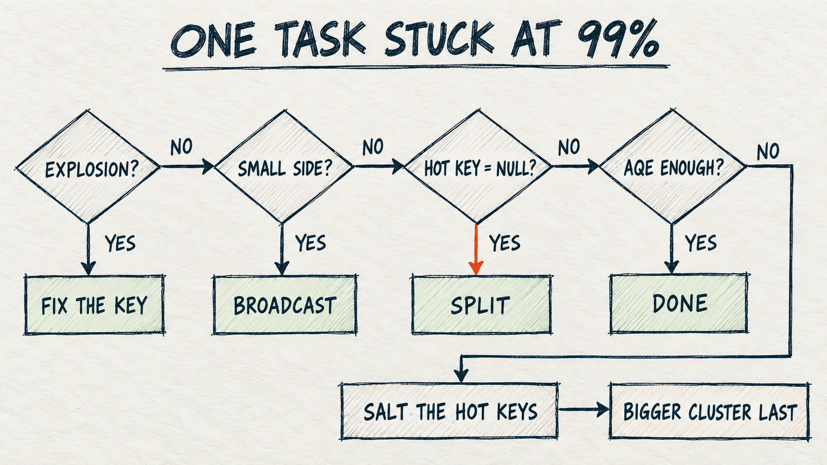
Problem
The symptom always looks similar. A job that usually takes a few minutes hangs on 199 of 200 tasks. One task has been running for a quarter of an hour, the others finished in seconds. Or the job fails with OOM on one executor while the rest of the cluster has free memory.
A typical skew demo is built on purpose: 90% of the fact rows get one customer key. That shows the mechanism well, but the most common trap lies elsewhere. Someone hears "skew", immediately pastes salting from the internet, and the real cause was a join explosion or thousands of empty keys that only needed filtering out.
Popular skew advice repeats two mistakes. A typical "Skew Solutions" table recommends "repartition() + salting" for a skewed groupBy, and a common line about NULL keys says that "NULLs never match in inner/left join anyway". The first does not help, and the second is only true for an inner join. I explain both in the tree.
In one project the most skewed key was client_id: one client had 800k orders while the others had around 20k each. The fix then goes in two steps, exactly as in the tree below: first AQE, which splits the skewed partition of a join on its own, and only when that isn't enough, salting just the hot key.
How it works
A shuffle distributes rows across partitions by the hash of the key. All rows with the same key land in the same partition, and one partition is processed by one task. If the key CUST000001 holds 90% of the rows, one task gets 90% of the work, no matter how many cores we have.
Spark has three built-in mechanisms for this, and it is worth knowing their limits:
| Mechanism | What it does | What it does not do |
|---|---|---|
| AQE skew join | Splits an oversized join partition into several tasks and duplicates the matching partition of the other side for them | Works only for joins with a shuffle. The partition must be both 5× larger than the median and larger than 256 MB (default thresholds) |
| Partial aggregation | A groupBy with sum, count, max computes a partial result in each task before the shuffle, so the hot key sends one row per task |
Does not help with aggregations that cannot be combined from parts: collect_list, exact percentiles, window functions |
| Broadcast join | The small side goes whole to every executor, the large side is not shuffled | Requires one side to be small (the default automatic threshold is 10 MB) |
The table leads to a conclusion that is easy to miss: on small data AQE will not treat a partition as skewed, even if it has 90% of the rows. If the whole table is 100 MB, no partition will exceed 256 MB. Skew on small data simply does not hurt, and on large data AQE has often already solved it. The problem lives in the middle: a few GB on the hot key, an aggregation that cannot be split, or an outer join.
The decision tree
0. Is it really skew?
Three problems look similar in the logs but are fixed in completely different ways:
- Join explosion. The join's output row count is many times larger than its input. All tasks are slow, not one. The fix is the join key, not compute.
- Spill in all tasks. Partitions are too big for memory, but even. More partitions or less volume after earlier filtering helps.
- Skew. One task (or a few) takes many times longer than the median.
On a classic cluster we check this in the Spark UI: the Stages tab, the slowest stage, "Summary metrics for tasks", and the max compared with the median. Serverless has no such tab, and the query profile shows per-operator metrics without the task distribution. Then we ask the data directly:
✓ Works on Free Edition
SELECT customer_id,
       count(*)                                         AS cnt,
       round(100 * count(*) / sum(count(*)) OVER (), 2) AS pct
FROM retailhub_demo.bronze.skew_facts
GROUP BY customer_id
ORDER BY cnt DESC
LIMIT 20;
If the first row holds tens of percent and the second a fraction of a percent, we have a hot key. If the first row is NULL, we go straight to step 3.
In the lab (29.09.2026, serverless), on the synthetic data generated by the notebook (2M facts, 10,000 customers), the result was: CUST000001 has 1,800,024 rows (90.0%), second place goes to NULL with 39,939 rows (2.0%), and the next customer has only 34 rows. That picture is both a hot key and a candidate for step 3.
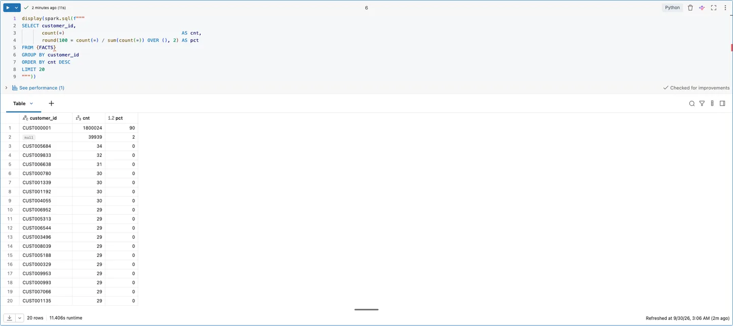
Lab result (Databricks, 29.09.2026): one key holds 90% of the rows, and the runner-up is NULL with 2%.
1. Where does the hot key live?
The same key can hurt in different operations, and each has a different remedy:
- join → steps 2–5,
groupBy→ step 6,- a window function with
PARTITION BYon the hot key → step 6, - source files (one 10 GB file next to a hundred 100 MB ones) or the partition for the last month → step 7.
2. Is one side of the join small?
If so, a broadcast fixes the problem at the root, because the large side does not go through a shuffle and there is no hot partition. AQE switches the join to broadcast by itself when a side turns out to be small after filters, but we can force it with a hint. On serverless this is the only way, because the autoBroadcastJoinThreshold cannot even be read there.
✓ Works on Free Edition
SELECT /*+ BROADCAST(d) */ f.*, d.segment
FROM retailhub_demo.bronze.skew_facts f
JOIN retailhub_demo.bronze.skew_dim d ON f.customer_id = d.customer_id;
In the lab (29.09.2026) the plan with the hint showed a PhotonBroadcastHashJoin with no shuffle on the fact side, and the join returned 1,960,061 rows, i.e. 2M minus the NULL rows.
The limit is simple: the broadcast side must fit in the memory of every executor. A dimension with millions of wide rows is already an OOM risk on the driver and executors.
3. Is the hot key NULL?
This is the most common "skew" that needs no salting at all. The behaviour depends on the join type:
- Inner join. The optimiser adds an
isnotnull(key)filter on both sides by itself, because NULL can never satisfy an equality condition. Rows with NULL never reach the shuffle. It is worth checking this in the plan instead of adding the filter blindly. - Left, right and full outer joins. Rows with NULL must stay in the result, so they go through the shuffle and all land in one partition. This is where the source comment was wrong: in a left join NULLs do not match, but they do not disappear either.
The fix for an outer join: cut the NULLs off before the join and append them back with empty dimension columns.
✓ Works on Free Edition
from pyspark.sql import functions as F

facts = spark.table("retailhub_demo.bronze.skew_facts")
dim   = spark.table("retailhub_demo.bronze.skew_dim")

nulls    = facts.filter(F.col("customer_id").isNull())
nonnulls = facts.filter(F.col("customer_id").isNotNull())

dim_cols = [c for c in dim.columns if c != "customer_id"]
left_joined = (
    nonnulls.join(dim, "customer_id", "left")
    .unionByName(nulls.select("*", *[F.lit(None).cast(dim.schema[c].dataType).alias(c)
                                     for c in dim_cols]))
)
Correctness check: left_joined.count() must equal facts.count() if the key is unique in the dimension. In the lab (29.09.2026) both versions, the split one and the plain left join, returned 2,000,000 rows each. The inner join plan had the isnotnull(customer_id) filter on both sides, with the broadcast and with the sort-merge join alike, so the 39,939 NULLs were dropped before the shuffle. The same problem applies to a groupBy on a column with many NULLs: the NULL group is one group and one task.
4. Is AQE already coping?
AQE is on by default on Databricks, and always on serverless. If the hot partition exceeds the thresholds from the table above, AQE splits it by itself. On a classic cluster this is visible in the Spark UI query plan (the node reading the shuffle reports skewed partitions), and we can lower the thresholds. On serverless we cannot change them, and in the lab (29.09.2026) we could not even read them: spark.conf.get raised AnalysisException for all four AQE settings, including spark.sql.adaptive.enabled. The only sign that AQE is active is the plan, which starts with AdaptiveSparkPlan.

Lab result (Databricks, 29.09.2026): on serverless the AQE thresholds cannot be read with spark.conf.get, so their defaults cannot be checked there either.
The practical takeaway: if a job hangs on one task even though AQE is on, then either the operation is not a join, or the partition does not exceed the threshold, or AQE split it and the hot key is still too big for one set of tasks. Then we move on to salting.
5. Salting: hot keys only
Salting breaks a hot key into N sub-keys. On the fact side, every row of the hot key gets a random salt from 0 to N−1. On the dimension side, that key's row is duplicated N times, once per salt. The join runs on the pair (key, salt). The source material gives a rough threshold: salting makes sense when AQE is not enough and the key imbalance exceeds 100:1.
We salt only the hot keys, because duplicating the whole dimension N times means N times more data on the other side of the join.
✓ Works on Free Edition
N = 16
hot_keys = [r["customer_id"] for r in
            facts.groupBy("customer_id").count()
                 .filter("count > 100000").select("customer_id").collect()]

facts_s = facts.withColumn(
    "salt",
    F.when(F.col("customer_id").isin(hot_keys), (F.rand() * N).cast("int"))
     .otherwise(F.lit(0)))

dim_s = (dim.withColumn(
            "salts",
            F.when(F.col("customer_id").isin(hot_keys), F.sequence(F.lit(0), F.lit(N - 1)))
             .otherwise(F.array(F.lit(0))))
            .withColumn("salt", F.explode("salts"))
            .drop("salts"))

salted = facts_s.join(dim_s.hint("merge"), ["customer_id", "salt"]).drop("salt")
The merge hint forces a sort-merge join here, so that with a small dimension the demo does not turn into a broadcast. In a real salting case both sides are large and the hint is not needed. We check the result by row count: the salted join must return as many rows as the plain one.
In the lab (29.09.2026, serverless) the hot key list had one element, CUST000001. Both joins returned 1,960,061 rows; the plain sort-merge join took 1.2 s and the salted one 1.3 s. On 2M rows that difference is noise, which matches the point from the table: on small data skew simply does not hurt. Where salting does show is the distribution: instead of 1,800,024 rows under one key we get 16 (key, salt) pairs with about 112k rows each (from 111,829 to 113,031 rows for each of the 16 salt values). We cannot read task counts on serverless, because there is no Stages tab. On top of that, the initial sort-merge join plan shuffled into 21 partitions, not 200, and Photon reported the SortMergeJoin node as unsupported, so the hint-forced join itself runs outside Photon.
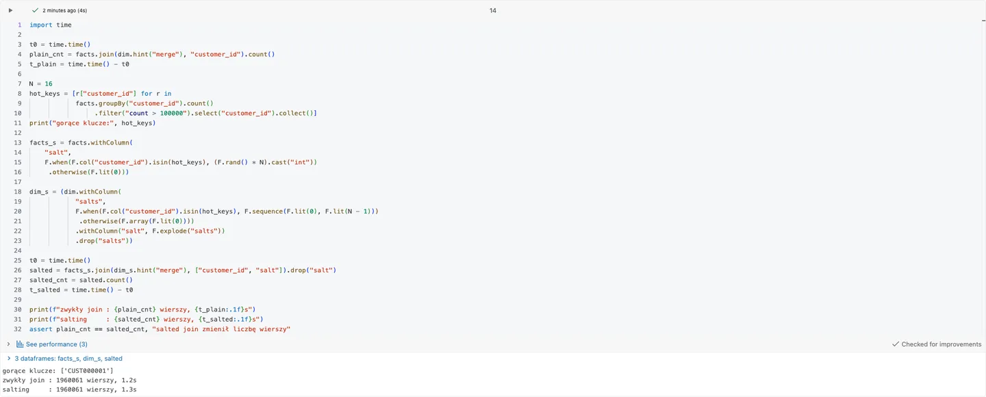
Lab result (Databricks, 29.09.2026): salting does not change the row count, and on 2M rows it does not change the time either.
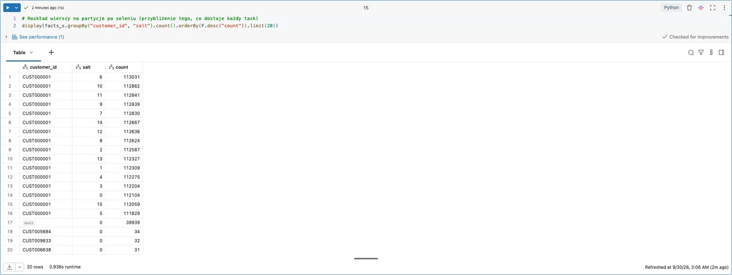
Lab result (Databricks, 29.09.2026): the hot key spreads evenly over 16 sub-keys, roughly 1/16 of its rows each.
Salting costs three things: code to maintain, a list of hot keys that changes over time, and duplicated rows in the dimension. That is why it sits so late in the tree.
6. Skewed groupBy and window functions
The popular "repartition() + salting" recommendation does not work for groupBy: groupBy shuffles by the key anyway, so an earlier repartition is either ignored or adds one more shuffle. The right question is: can the aggregation be combined from parts?
sum,count,min,max,avg. Partial aggregation already does this. A skewedgroupBywith these functions is rarely a problem.count(DISTINCT x). We split it into two steps: first the unique pairs (key, x), then a plaincount. The first shuffle runs on the pair, so the hot key spreads across many partitions.- A window function on the hot key.
row_number() OVER (PARTITION BY customer_id ORDER BY ts)sorts all rows of the key in one task. If we only need the latest row per key,max_bydoes it as an aggregation with partial aggregation.
✓ Works on Free Edition
# count(DISTINCT product_id) per customer in two steps
distinct_products = (facts.select("customer_id", "product_id").distinct()
                          .groupBy("customer_id").count())

# latest order per customer without a window function
latest = (facts.groupBy("customer_id")
               .agg(F.max_by(F.struct(*facts.columns), F.col("order_ts")).alias("r"))
               .select("r.*"))
In the lab (29.09.2026) the two-step version gave exactly the same result as countDistinct (0 differences in exceptAll).
For collect_list on a hot key there is no good answer: the result is one huge array in one row anyway. Then we ask whether that array is needed at all.
7. Skew in the data on disk
One 10 GB source file next to a hundred 100 MB ones, or a table partitioned by date where the last month is an order of magnitude larger, produce skewed tasks already at read time. Here OPTIMIZE and Liquid Clustering instead of static partitioning help.
8. A bigger cluster: last
More executors do not help, because the hot partition still goes to one task. A bigger node may help with OOM, but it treats the symptom. One line sums it up: fix the key, not the cluster.
Pitfalls
- Salting the whole key space. Duplicating the whole dimension N times can cost more than the skew it was meant to fix. We salt only the keys on the hot list.
- Salt from
rand()without checking the result. After changing a join we always compare the row count with the plain join. A mistake in the join condition (e.g.saltmissing on one side) gives a silent explosion. - A hard-coded hot key list. Data distribution changes. We compute the list in the job or keep it in a configuration table.
- Tuning AQE thresholds on serverless. Not possible. Hints and rewriting the query remain.
- Measuring on small data. On a few million rows AQE will not even treat a partition as skewed, and timing differences are in the noise (in the lab: 1.2 s vs 1.3 s on 2M rows). We count tasks and rows per partition.
- Hunting skew when the problem is an explosion. First compare the join's input and output rows.
When NOT to use it
We do not apply salting or manual aggregation splitting "just in case". If the job finishes in acceptable time, AQE and broadcast are usually enough, and manual optimisation is extra code to maintain. We also do not use them when the cause is a bad data model, e.g. a fact-to-fact join on a key that is unique in neither table. There the model has to change, not the query plan.
See it run
The recording walks through the lab notebook step by step: the key distribution, broadcast, NULLs in the inner and left join, salting and the groupBy rewrite.
The full notebook is in code/data_skew.py. The data is synthetic and generated in the notebook, so you can reproduce the results on your own workspace.
Summary
- Before calling a problem skew, we rule out a join explosion and even spill.
- Serverless has no task distribution, so we check the key distribution with a
GROUP BY ... ORDER BY cnt DESCquery. - Order of fixes: broadcast, handling NULLs in outer joins, AQE, salting hot keys only, rewriting aggregations and windows. A bigger cluster last.
- AQE splits only join partitions above the thresholds (by default 5× the median and 256 MB), so it will not help with
groupBy, windows or small data. - Fix the key, not the cluster.
As of:
Want more posts? Follow along via RSS or on LinkedIn.

Comments
Quiet on the trail so far. Be the first to comment.